Color and Gradient

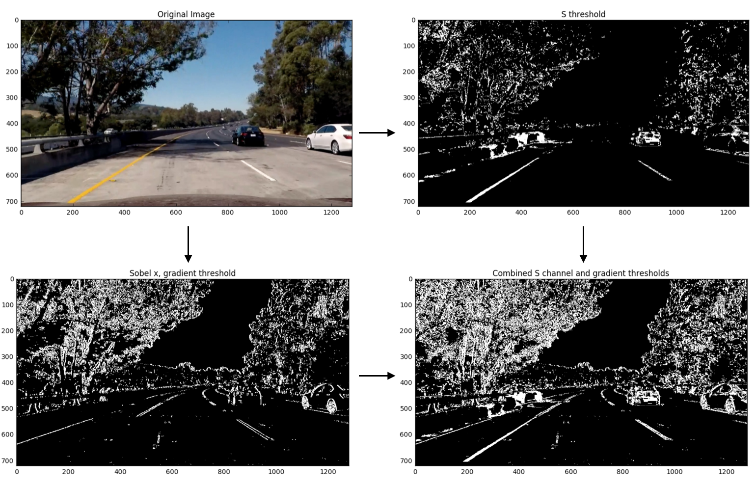
Now it's time to combine what you know about color and gradient thresholding to get the best of both worlds. Here's an example of how that might look:

At this point, it's okay to detect edges around trees or cars because these lines can be mostly filtered out by applying a mask to the image and essentially cropping out the area outside of the lane lines. It's most important that you reliably detect different colors of lane lines under varying degrees of daylight and shadow.

You can clearly see which parts of the lane lines were detected by the gradient threshold and which parts were detected by the color threshold by stacking the channels and seeing the individual components. You can create a binary combination of these two images to map out where either the color or gradient thresholds were met.

Here's what that looks like in code:

# Convert to HLS color space and separate the S channel
# Note: img is the undistorted image
hls = cv2.cvtColor(img, cv2.COLOR_RGB2HLS)
s_channel = hls[:,:,2]

# Grayscale image
# NOTE: we already saw that standard grayscaling lost color information for the lane lines
# Explore gradients in other colors spaces / color channels to see what might work better
gray = cv2.cvtColor(img, cv2.COLOR_RGB2GRAY)

# Sobel x
sobelx = cv2.Sobel(gray, cv2.CV_64F, 1, 0) # Take the derivative in x
abs_sobelx = np.absolute(sobelx) # Absolute x derivative to accentuate lines away from horizontal
scaled_sobel = np.uint8(255*abs_sobelx/np.max(abs_sobelx))

# Threshold x gradient
thresh_min = 20
thresh_max = 100
sxbinary = np.zeros_like(scaled_sobel)
sxbinary[(scaled_sobel >= thresh_min) & (scaled_sobel <= thresh_max)] = 1

# Threshold color channel
s_thresh_min = 170
s_thresh_max = 255
s_binary = np.zeros_like(s_channel)
s_binary[(s_channel >= s_thresh_min) & (s_channel <= s_thresh_max)] = 1

# Stack each channel to view their individual contributions in green and blue respectively
# This returns a stack of the two binary images, whose components you can see as different colors
color_binary = np.dstack(( np.zeros_like(sxbinary), sxbinary, s_binary)) * 255

# Combine the two binary thresholds
combined_binary = np.zeros_like(sxbinary)
combined_binary[(s_binary == 1) | (sxbinary == 1)] = 1

# Plotting thresholded images
f, (ax1, ax2) = plt.subplots(1, 2, figsize=(20,10))
ax1.set_title('Stacked thresholds')
ax1.imshow(color_binary)

ax2.set_title('Combined S channel and gradient thresholds')
ax2.imshow(combined_binary, cmap='gray')

The output is shown below. The final image color_binary is a combination of binary thresholding the S channel (HLS) and binary thresholding the result of applying the Sobel operator in the x direction on the original image.

In this next exercise, you'll get the chance to play around with different combinations of color and gradient with the goal using the pipeline you come up with for your upcoming project. There's no correct submission, just explore!

Some interesting things to explore might include: the H channel, different threshold values for color and gradient binary images, and even a different color space, like HSV!

You can download the image used in the quiz here .

Start Quiz:

import numpy as np
import cv2
import matplotlib.pyplot as plt
import matplotlib.image as mpimg


image = mpimg.imread('bridge_shadow.jpg')

# Edit this function to create your own pipeline.
def pipeline(img, s_thresh=(170, 255), sx_thresh=(20, 100)):
    img = np.copy(img)
    # Convert to HLS color space and separate the V channel
    hls = cv2.cvtColor(img, cv2.COLOR_RGB2HLS)
    l_channel = hls[:,:,1]
    s_channel = hls[:,:,2]
    # Sobel x
    sobelx = cv2.Sobel(l_channel, cv2.CV_64F, 1, 0) # Take the derivative in x
    abs_sobelx = np.absolute(sobelx) # Absolute x derivative to accentuate lines away from horizontal
    scaled_sobel = np.uint8(255*abs_sobelx/np.max(abs_sobelx))
    
    # Threshold x gradient
    sxbinary = np.zeros_like(scaled_sobel)
    sxbinary[(scaled_sobel >= sx_thresh[0]) & (scaled_sobel <= sx_thresh[1])] = 1
    
    # Threshold color channel
    s_binary = np.zeros_like(s_channel)
    s_binary[(s_channel >= s_thresh[0]) & (s_channel <= s_thresh[1])] = 1
    # Stack each channel
    color_binary = np.dstack(( np.zeros_like(sxbinary), sxbinary, s_binary)) * 255
    return color_binary
    
result = pipeline(image)

# Plot the result
f, (ax1, ax2) = plt.subplots(1, 2, figsize=(24, 9))
f.tight_layout()

ax1.imshow(image)
ax1.set_title('Original Image', fontsize=40)

ax2.imshow(result)
ax2.set_title('Pipeline Result', fontsize=40)
plt.subplots_adjust(left=0., right=1, top=0.9, bottom=0.)